Coinbase Pro (formerly known as GDAX) is one of the biggest cryptocurrency exchange, you can trade a large panel of cryptocurrencies against USD, EUR and GBP. I chose to trade on Coinbase Pro because it supports a lot of pairs and the liquidity is usually very good, we can easily implement an algorithmic trading strategy on this exchange.
The most traded currencies are: – Bitcoin (BTC) – Ethereum (ETH) – yearn.finance (YFI) – Litecoin (LTC)
The Setup
Fortunately for us, Coinbase Pro provides an API to get market data, to get balances for each currency and to send buy/sell orders to the market. You can find a documentation here.
I found a Python wrapper for their API on GitHub, this one is super easy to use. You can install the package like this:
pip install cbpro
Once it’s installed, you need to insert the appropriate import in your code:
import cbpro
Now you need to get an API key in order to be able to retrieve your account balances and to send orders to the market. If you just want to get market data you can skip that part. Go to https://pro.coinbase.com/profile/api , click on Create new key, now you have the API key and you may need to get some email validation to see the secret key (which you also need). Check the options you want, if you want to trade via the API, just select the appropriate check box, same for withdrawals.
Using the API
In your code, you need to set up the connection so that you can get authenticated:
With this basic API you can code any algorithmic strategy in Python for Coinbase Pro, you can try to predict the value of a cryptocurrency using our previoustutorials for example.
This one is the most important, before starting anything you should learn about programming. Coding will make you assimilate a certain logic that’s close to mathematical formulas and can help you formalize your trading process. It’s essential to be able to understand everything that’s “under the hood”, what if you strategy starts to slow down after a few months and you’re not able to improve it yourself.
You won’t learn programming in a day, you should take your time to learn and understand the process. Fortunately, there are multiple free methods you can use to learn about Python. You can use websites like EDX, Coursera, and Udacity.
#2 Backtesting and training on the same period
Let’s say you found the perfect strategy that makes +300% in the 2014 period, you may want to backtest it on a different period, the strategy may work in that specific time but it could make you lose a lot on another period. This beginner mistake has a name: overfitting. Ideally you want to split your data set into at least 2 parts: train and test. But if you want to have a rock-solid performance, you can try K-Fold cross validation, it’ll split your data set into K parts, train 1 part and test it on the other ones, and so on.
#3 Not backtesting enough
Backtest, backtest and backtest. Use different time periods, adjust the trading size, the strategy could work by buying 100$ worth of stocks at a time but what if you want to scale it ? You could introduce slippage and of course broker fees.
Backtesting is good but paper trading is better, you should run the strategy in real-time but without any broker connection, this way you can simulate how it’s going to behave with current market situation.
#4 Not having a risk management strategy
Risk management is going to make a difference during bear markets or high-volatility periods. You can limit the maximum exposure and ignore any buying signal if you hit the limit, or automatically close any position older than a few days. These are suggestions, it’s important to make sure you won’t get stuck with a growing loss over time.
#5 Having unreliable data
Your strategy will be based on financial data, either real-time, minute or daily data, a single data point can destroy your profits. You need to make sure it’s coming from a reliable source and not some random websites, a good source is Quandl, some of their datasets are free.
Zipline is a backtesting engine for Python, if you’re a Quantopian member you should be familiar with it since it’s the one they’re using. It provides metrics about the strategy such as returns, standard deviations, Sharpe ratios etc. basically everything you need to know in order to validate or not a strategy before going live.
Zipline can be install using pip:
pip install zipline
If you’re on Windows I suggest using Conda:
conda install -c Quantopian zipline
Here is the basic structure of a strategy in Zipline:
from zipline.api import order, record, symbol

def initialize(context):
    pass

def handle_data(context, data):
    order(symbol('AAPL'), 10)
    record(AAPL=data.current(symbol('AAPL'), 'price'))
In initialize you can set some global variables used for the strategy such as a list of stocks, certain parameters, the maximum percentage of portfolio invested. Then handle_data is entered at every tick, that’s where your strategy logic should be. You can check previous articles and incorporate strategies into your code.
Let’s breakdown the handle_data()code.
The order() function let you create an order, here we specify the AAPL ticker (Apple stock) with a quantity of 10. A positive value means you’re buying 10 stocks, a negative value would mean you’re selling the stock.
Then, the record() function allows you to save the value of a variable at each iteration. Here, you’re saving the current stock price under the variable named AAPL, you’ll then be able to retrieve that information in the backtest result, this way you can compare your strategy performance versus the stock price.
Now you want to finally backtest the strategy and see if it’s profitable. To do that, run the following command:
This command is going to run the backtest between 2015-01-01 and 2020-01-01 and output the result into a pickle file for later analysis. The pickle is simply a Pandas DataFrame with a line per day and (a lot of) columns regarding your strategy, such as the return, the number of orders, the portofolio size and so on.
Random Forest is a powerful machine learning algorithm, it can be used as a regressor or as a classifier. It’s a meta estimator, meaning it’s using a specified number of decision trees to fit and predict.
We’re going to use the package Scikit-Learn in Python, it’s a very useful library which contains a lot of machine learning algorithms and related tools.
Data preparation
To see how Random Forest can be applied, we’re going to try to predict the S&P 500 futures (E-Mini), you can get the data for free on Quandl. Here is what it looks like:
[table] Date,Open,High,Low,Last,Change,Settle,Volume,Previous Day Open Interest
2016-12-30,2246.25,2252.75,2228.0,2233.5,8.75,2236.25,1252004.0,2752438.0
2016-12-29,2245.5,2250.0,2239.5,2246.25,0.25,2245.0,883279.0,2758174.0
2016-12-28,2261.25,2267.5,2243.5,2244.75,15.75,2245.25,976944.0,2744092.0[/table]
The column Change needs to be removed since there’s missing data and this information can be retrieved directly by substracting D close and D-1 close.
Since it’s a classifier, we need to create classes for each line: 1 if the future went up today, -1 if it went down or stayed the same.
import numpy as np
import pandas as pd

def computeClassification(actual):
if(actual > 0):
return 1
else:
return -1

data = pd.DataFrame.from_csv(path='EMini.csv', sep=',')

# Compute the daily returns
data['Return'] = (data['Settle']/data ['Settle'].shift(-1)-1)*100

# Delete the last line which contains NaN
data = data.drop(data.tail(1).index)

# Compute the last column (Y) -1 = down, 1 = up
data.iloc[:,len(data.columns)-1] = data.iloc[:,len(data.columns)-1].apply(computeClassification)
Now that we have a complete dataset with a predictable value, the last colum “Return” which is either -1 or 1, let’s create the train and test dataset.
testData = data[-(len(data)/2):] # 2nd half
trainData = data[:-(len(data)/2)] # 1st half

# X is the list of features (Open, High, Low, Settle)
data_X_train = trainData.iloc[:,0:len(trainData.columns)-1]
# Y is the value to be predicted
data_Y_train = trainData.iloc[:,len(trainData.columns)-1]

# Same thing for the test dataset
data_X_test = testData.iloc[:,0:len(testData.columns)-1]
data_Y_test = testData.iloc[:,len(testData.columns)-1]
Using the algorithm
Once we have everything ready we can start fitting the Random Forest classifier against our train dataset:
from sklearn import ensemble

# I picked 100 randomly, we'll see in another post how to find the optimal value for the number of estimators
clf = ensemble.RandomForestClassifier(n_estimators = 100, n_jobs = -1)
clf.fit(data_X_train, data_Y_train)

predictions = clf.predict(data_X_test)
predictions is an array containing the predicted values (-1 or 1) for the features in data_X_test.
You can see the prediction accuracy using the method accuracy_score which compares the predicted values versus the expected ones.
from sklearn.metrics import accuracy_score

print "Score: "+str(accuracy_score(data_Y_test, y_predictions))
What’s next ?
Now for example you can create a trading strategy that goes long the future if the predicted value is 1, and goes short if it’s -1. This can be easily backtested using a backtest engine such as Zipline in Python.
Based on your backtest result you could add or remove features, maybe the volatility or the 5-day moving average can improve the prediction accuracy ?
Finding trading signals is one of the core problems of algorithmic trading, without any good signals your strategy will be useless. This is a very abstract process as you cannot intuitively guess what signals will make your strategy profitable or not, because of that I’m going to explain how you can have at least a visualization of the signals so that you can see if the signals make sense and introduce them in your algorithm.
We’re going to use matplotlib to graph the asset price and add buy/sell signals on the same graph, this way you can see if the signals are generated at the right moment or not: buy low, sell high.
Data preparation
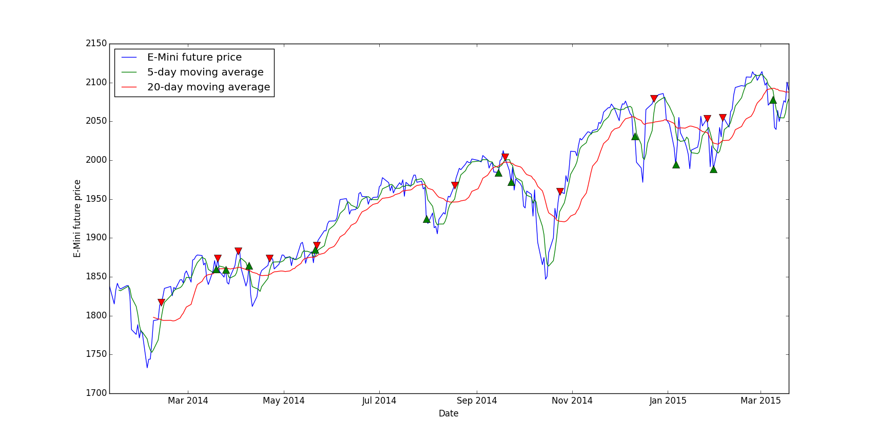
For this tutorial I picked a very simple strategy which is a crossing moving average, the idea is to buy when the “short” moving average, let’s say 5-day is crossing the “long” moving average, let’s say 20-day, and to sell when they cross the other way.
First of all, we need to install matplotlib via the usual pip:
pip install matplotlib
This example requires pandas and matplotlib:
import pandas as pd
import matplotlib.pyplot as plt
Loading data and computing the moving averages is pretty trivial thanks to Pandas:
data = pd.DataFrame.from_csv(path='EMini.csv', sep=',')

# Generate moving averages
data = data.reindex(index=data.index[::-1]) # Reverse for the moving average computation
data['Mavg5'] = data['Settle'].rolling(window=5).mean()
data['Mavg20'] = data['Settle'].rolling(window=20).mean()
Now the actual signal generation part is a bit more tricky:
# Save moving averages for the day before
prev_short_mavg = data['Mavg5'].shift(1)
prev_long_mavg = data['Mavg20'].shift(1)

# Select buying and selling signals: where moving averages cross
buys = data.ix[(data['Mavg5'] <= data['Mavg20']) & (prev_short_mavg >= prev_long_mavg)]
sells = data.ix[(data['Mavg5'] >= data['Mavg20']) & (prev_short_mavg <= prev_long_mavg)]
buys and sells is now containing all dates where we have a signal.
Plotting the signals
The interesting part is the graphing of this, the syntax is simple:
plt.plot(X, Y)
We want to display the E-Mini price and the moving averages is pretty simple, we use data.index because the dates in the DataFrame are in the index:
# The label parameter is useful for the legend
plt.plot(data.index, data['Settle'], label='E-Mini future price')
plt.plot(data.index, data['Mavg5'], label='5-day moving average')
plt.plot(data.index, data['Mavg20'], label='20-day moving average')
But for the signals, we want to put each marker at the specific date, which is in the index, and at the E-Mini price level so that visually it’s not too confusing:
In conclusion, you can interpret this by noticing that most buying signals are at dips in the curve and selling signals are at local maximums. So our signal generation looks promising, however without a real backtest we cannot be sure that the strategy will be profitable, at least we can validate or not a signal. The main advantage of this method is that we can instantly see if the signals are “right” or not, for example you can play with the short and long moving average, you could try 10-day versus 30-day etc. and in the end you can pick the right parameters for this signal.
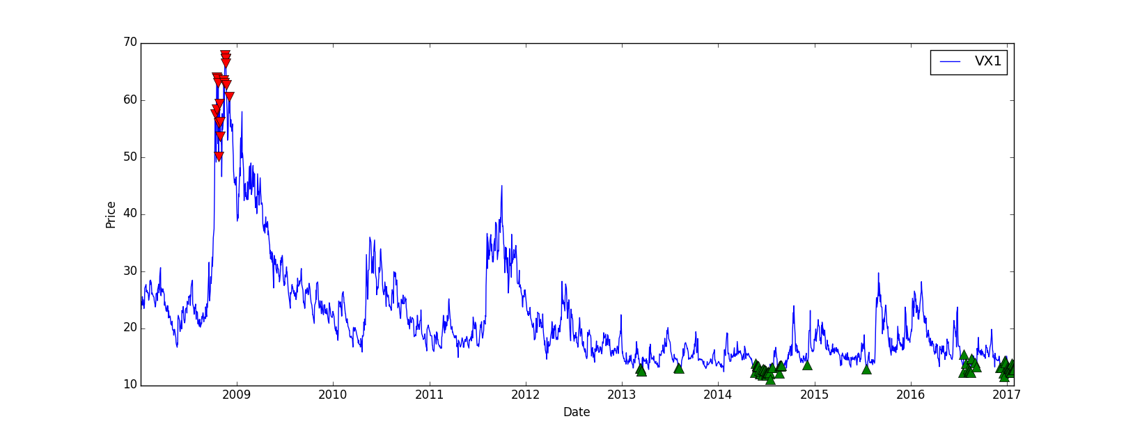
To show you the full process of creating a trading strategy, I’m going to work on a super simple strategy based on the VIX and its futures. I’m just skipping the data downloading from Quandl, I’m using the VIX index from here and the VIX futures from here, only the VX1 and VX2 continuous contracts datasets.
Data loading
First we need to load all the necessary imports, the backtest import will be used later:
import pandas as pd
import numpy as np
import matplotlib.pyplot as plt
from backtest import backtest
from datetime import datetime
For the sake of simplicity, I’m going to put all values in one DataFrame and in different columns. We have the VIX index, VX1 and VX2, this gives us this code:
VIX = "VIX.csv"
VIX1 = "VX1.csv"
VIX2 = "VX2.csv"

data = []
fileList = []
# Create the base DataFrame
data = pd.DataFrame()

fileList.append(VIX)
fileList.append(VIX1)
fileList.append(VIX2)

# Iterate through all files
for file in fileList:
# Only keep the Close column
tmp = pd.DataFrame(pd.DataFrame.from_csv(path=file, sep=',')['Close'])

# Rename the Close column to the correct index/future name
tmp.rename(columns={'Close': file.replace(".csv", "")}, inplace=True)

# Merge with data already loaded
# It's like a SQL join on the dates
data = data.join(tmp, how = 'right')

# Resort by the dates, in case the join messed up the order
data = data.sort_index()
And here’s the result:
[table]
Date,VIX,VX1,VX2
02/01/2008,23.17,23.83,24.42
03/01/2008,22.49,23.30,24.60
04/01/2008,23.94,24.65,25.37
07/01/2008,23.79,24.07,24.79
08/01/2008,25.43,25.53,26.10
[/table]
Signals
For this tutorial I’m going to use a very basic signal, the structure is the same and you can replace the logic with your whatever strategy you want, using very complex machine learning algos or just crossing moving averages.
The VIX is a mean-reverting asset, at least in theory, it means it will go up and down but in the end its value will move around an average. Our strategy will be to go short when it’s way higher than its mean value and to go short when it’s very low, based on absolute values to keep it simple.
high = 65
low = 12

# By default, set everything to 0
data['Signal'] = 0

# For each day where the VIX is higher than 65, we set the signal to -1 which means: go short
data.loc[data['VIX'] > high, 'Signal'] = -1

# Go long when the VIX is lower than 12
data.loc[data['VIX'] < low, 'Signal'] = 1

# We store only days where we go long/short, so that we can display them on the graph
buys = data.ix[data['Signal'] == 1]
sells = data.ix[data['Signal'] == -1]
Now we’d like to visualize the signal to check if, at least, the strategy looks profitable:
# Plot the VX1, not the VIX since we're going to trade the future and not the index directly
plt.plot(data.index, data['VX1'], label='VX1')
# Plot the buy and sell signals on the same plot
plt.plot(sells.index, data.ix[sells.index]['VX1'], 'v', markersize=10, color='r')
plt.plot(buys.index, data.ix[buys.index]['VX1'], '^', markersize=10, color='g')
plt.ylabel('Price')
plt.xlabel('Date')
plt.legend(loc=0)
# Display everything
plt.show()
The result is quite good, even though there’s no trade between 2009 and 2013, we could improve that later:
Backtesting
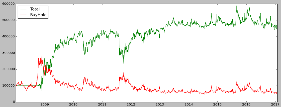
Let’s check if the strategy is profitable and get some metrics. We’re going to compare our strategy returns with the “Buy and Hold” strategy, which means we just buy the VX1 future and wait (and roll it at each expiry), this way we can see if our strategy is more profitable than a passive one.
I put the backtest method in a separate file to make the main code less heavy, but you can keep the method in the same file:
import numpy as np
import pandas as pd

# data = prices + dates at least
def backtest(data):
cash = 100000
position = 0
total = 0

data['Total'] = 100000
data['BuyHold'] = 100000
# To compute the Buy and Hold value, I invest all of my cash in the VX1 on the first day of the backtest
positionBeginning = int(100000/float(data.iloc[0]['VX1']))
increment = 1000

for row in data.iterrows():
price = float(row[1]['VX1'])
signal = float(row[1]['Signal'])

if(signal > 0 and cash - increment * price > 0):
# Buy
cash = cash - increment * price
position = position + increment
print(row[0].strftime('%d %b %Y')+" Position = "+str(position)+" Cash = "+str(cash)+" // Total = {:,}".format(int(position*price+cash)))

elif(signal < 0 and abs(position*price) < cash):
# Sell
cash = cash + increment * price
position = position - increment
print(row[0].strftime('%d %b %Y')+" Position = "+str(position)+" Cash = "+str(cash)+" // Total = {:,}".format(int(position*price+cash)))

data.loc[data.index == row[0], 'Total'] = float(position*price+cash)
data.loc[data.index == row[0], 'BuyHold'] = price*positionBeginning

return position*price+cash
In the main code I’m going to use the backtest method like this:
It’s important to display the annualized return, a strategy with a 20% return over 10 years is different than a 20% return over 2 months, we annualize everything so that we can compare strategies easily. The Sharpe Ratio is a useful metric, it allows us to see if the return is worth the risk, in this example I just assumed a 0% risk-free rate, if the ratio is > 1 it means the risk-adjusted return is interesting, if it’s > 10 it means the risk-adjusted return is very interesting, basically high return for a low volatility.
In our example we have a pretty nice Sharpe ratio of 4.6 which is quite good:
The strategy perfomed very well until 2010 but then from 2013 the PnL starts to stagnate:
Backtest
Conclusion
I showed you a basic structure of creating a strategy, you can adapt it to your needs, for example you can implement your strategy using zipline instead of a custom bactktesting module. With zipline you’ll have way more metrics and you’ll easily be able to run your strategy on different assets, since market data is managed by zipline.
I didn’t mention any transactions fees or bid-ask spread in this post, the backtest doesn’t take into account all of this so maybe if we include them the strategy would lose money!
Poloniex is a cryptocurrency exchange, you can trade ~80 cryptocurrencies against Bitcoin and a few others against Ethereum. I chose to trade on Poloniex because it supports a lot of currencies and the liquidity is usually very good, we can easily implement an algorithmic trading strategy on this exchange.
The most traded currencies are:
– Bitcoin (BTC)
– Ethereum (ETH)
– Monero (XMR)
– Tether (USDT)
The Setup
Fortunately for us, Poloniex provides an API to get market data, to get balances for each currency and to send buy/sell orders to the market. You can find a documentation here.
I found a Python wrapper for their API on GitHub, this one is super easy to use.
You can install the package like this:
Once it’s installed, you need to insert the appropriate import in your code:
from poloniex import Poloniex
Now you need to get an API key in order to be able to retrieve your account balances and to send orders to the market. If you just want to get market data you can skip that part.
Go to https://poloniex.com/apiKeys , click on Create new key, now you have the API key and you may need to get some email validation to see the secret key (which you also need). Check the options you want, if you want to trade via the API, just select the appropriate check box, same for withdrawals.
Using the API
In your code, you need to set up the connection so that you can get authenticated. You can just use the commented line if you only want to access the public API:
apiKey = "API_KEY"
secret = "SECRET_KEY"
polo = Poloniex(apiKey, secret)
# polo = Poloniex()
pair = "BTC_ETH"
price = 0.1
order = polo.buy("BTC_ETH", price, 1)
order = polo.sell("BTC_ETH", price, 1)
You’ll get an order object in JSON, resultingtrades is an array of trades generated by the order, the order can be filled straight away with multiple trades:
{‘orderNumber’: ‘0000000’, ‘resultingTrades’: []}
To manage your risks, you’ll need to retrieve your balances:
With this basic API you can code any algorithmic strategy in Python for Poloniex, you can try to predict the value of a cryptocurrency using our previoustutorials for example.
This article by Steven Buchko was originally published at CoinCentral.com
Whether you’re a crypto expert or just getting your feet wet with investing, there’s plenty to be aware of when trading your way through the cryptocurrency industry. Unlike in traditional markets, cryptocurrency trading is chock full of volatility, nefarious players, and irrational price movements.
In this article, we’ll teach you about some of the common mistakes in cryptocurrency trading and how you can avoid them.
Mistake #1: Chasing Pumps aka FOMO
Probably the most common (and easiest) mistake to make in cryptocurrency trading is buying into a coin after it’s already risen a significant amount. Investors that bought into Ripple (XRP) and Tron (TRX) at the peak of their runs in 2017 definitely felt the pain just a few weeks later in 2018. It may be your instinct to throw some money in the ring when you see a coin shoot up 30-40% because it’s “hot.” Don’t.
Extreme increases in price are almost always accompanied by some type of pullback. By the time you hear about a “hot” coin, it’s usually too late. Unless you’ve done your research, believe in the fundamentals of the coin, and want to hold it for the long-term (>1 year), wait until the pullback to invest.
Pump and Dumps
Pump and dumps (PnDs) are a special breed of pumps that are guaranteed to leave you burned. If you see an unknown coin skyrocket all of a sudden, be wary. It’s most likely part of a PnD scheme. They’re basically coordinated efforts to artificially drive up the price of a coin (the pump) before selling it to those who FOMO’d in (the dump).
When you come across a coin like this, the first thing to check is the trading volume. CoinMarketCap is a great resource for this. Any 24-hour trading volume under $1 million should raise a red flag.
Mistake #2: Not Knowing Your Investments
Don’t just blindly follow the advice of some Twitter or YouTube “guru” for investment picks. Many times, these high-profile individuals are paid to promote certain coins. Even John McAfee, one of the most well-known figures in the space admitted that he gets paid to promote projects. Question the coins that you’re told to invest in.
At the bare minimum, you should devote a half hour to researching any project in which you plan to invest in. Check out what problem it’s attempting to solve, the team building it, and the economics of the coin. Has the project partnered with anyone significant? Any notable names as advisors? These are all things you should know.
Even a quick Google search could unveil some information that turns what may seem like gold into trash. Taking it a step further, you should ideally read the white paper of each project you invest in.
Joining or forming an investment group can do wonders to help with this. It forces you to do research so you can explain your investment reasoning to your peers. It also puts you an environment in which you have to challenge your assumptions as others question your reasoning.
Mistake #3: Selling At Inappropriate Times
The opposite of chasing pumps, emotion-driven selling is still cut from the same cloth. It’s difficult, but you need to stay level-headed when trading – keep emotions out of it. Time and time again, coins have dipped down double-digit percentages before rocketing to 200-300% gains.
When a coin you own starts to drop in value, before you sell, re-evaluate your position. If you invested because you believe in the coin’s fundamentals, there are a few questions you can ask yourself:
Have any of the fundamentals changed?
Were there any announcements that would have affected the price?
Have you stopped believing in the long-term vision of the coin?
If your answer to all of these questions is “No”, then consider holding on. This strategy becomes much easier when you follow the golden rule of cryptocurrency trading: Don’t invest more money than you’re comfortable losing.
On the other side of this equation, seeing some solid gains may also tempt you to sell. Although taking profits is wise, you may want to avoid selling your entire stack. Depending on the situation, the coin could rise further. A popular trading strategy is to take out your initial investment while keeping your earnings invested in the coin after gaining a certain percentage. This decreases your downside risk while still exposing you to the upside potential.
Mistake #4: Being Uninformed
In a market that moves as rapidly as cryptocurrency does, you need to stay up-to-date with industry news. Without tuning in weekly, or even daily, the investment tides could shift without you even knowing.
Twitter, Reddit, and projects’ Telegram channels are also great resources you can use to stay informed. Oftentimes, teams share project updates and important announcements on these platforms before they hit mainstream media. Joining these communities also gives you the opportunity to be more involved with the projects while sometimes even impacting future development.
Good Luck Out There
Even with these tips, there’s bound to be mistakes that you make. Don’t let that discourage you – it happens to everyone. Part of the investing process is to learn from those mistakes and not make them again.
Continuous improvement is the name of the game. And, as long as you’ve got that going for you, you’ll be a trading whiz in no time.