How to convert a JSON into a HDF5 file

You scraped a bunch of data from a cryptocurrency exchange API into JSON but you figured that it’s taking too much disk space ? Switching to HDF5 will save you some space and make the access very fast, as it’s optimized for I/O operations. The HDF5 format is supported by major tools like Pandas, Numpy and Keras, data integration will be smooth, if you want to do some analysis.

Flattening the JSON

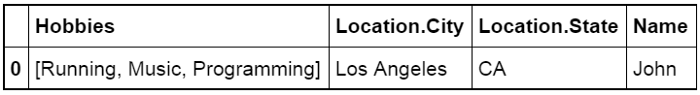
Most of the time JSON data is a giant dictionary with a lot of nested levels, the issue is that HDF5 doesn’t understand that. If we take the below JSON:

json_dict = {'Name':'John', 'Location':{'City':'Los Angeles','State':'CA'}, 'hobbies':['Music', 'Running']}

The result will look like this in a DataFrame:

Nested DataFrame
Nested DataFrame

We need to flatten the JSON to make it look like a classic table:

Flatten DataFrame
Flatten DataFrame

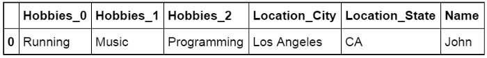
We’re going to use the flatten_json() function (more info here):

def flatten_json(y):
    out = {}

    def flatten(x, name=''):
        if type(x) is dict:
            for a in x:
                flatten(x[a], name + a + '_')
        elif type(x) is list:
            i = 0
            for a in x:
                flatten(a, name + str(i) + '_')
                i += 1
        else:
            out[name[:-1]] = x

    flatten(y)
    return out

Loading into a HDF5 file

Now the idea is to load the flattened JSON dictionary into a DataFrame that we’re going to save in a HDF5 file.

I’m assuming that during scraping we appended each record to the JSON, so we have one dictionary per line:

def json_to_hdf(input_file, output_file):
    
    with pd.HDFStore(output_file) as store:
        with open(input_file, "r") as json_file:
            for i, line in enumerate(json_file):
                try:
                    flat_data = flatten_json(ujson.loads(line))
                    df = pd.DataFrame.from_dict([flat_data])
                    store.append('observations', df)
                except:
                    pass

Let’s break this down.

Line 3: we initialize the HDFStore, this is the HDF5 file, it’s handling the file writing and everything.

Lines 4 & 5: we open the file and read it line per line

Line 7: we transform the line into a JSON dictionary and then we flatten it

Line 8: we transform the flatten dictionary into a Pandas DataFrame

Line 9: we append this DataFrame into the HDFStore

Et voilà, you now have your data in a single HDF5 file, ready to be loaded for your statistical analysis or maybe to generate trading signals, remember, it’s optimized for Pandas and Numpy so it’ll be faster than reading from the original JSON file.

Trading with Coinbase Pro (GDAX) API in Python

Coinbase Pro (formerly known as GDAX) is one of the biggest cryptocurrency exchange, you can trade a large panel of cryptocurrencies against USD, EUR and GBP. I chose to trade on Coinbase Pro because it supports a lot of pairs and the liquidity is usually very good, we can easily implement an algorithmic trading strategy on this exchange.

The most traded currencies are:
– Bitcoin (BTC)
– Ethereum (ETH)
– yearn.finance (YFI)
– Litecoin (LTC)

The Setup

Fortunately for us, Coinbase Pro provides an API to get market data, to get balances for each currency and to send buy/sell orders to the market. You can find a documentation here.

I found a Python wrapper for their API on GitHub, this one is super easy to use.
You can install the package like this:

pip install cbpro

Once it’s installed, you need to insert the appropriate import in your code:

import cbpro

Now you need to get an API key in order to be able to retrieve your account balances and to send orders to the market. If you just want to get market data you can skip that part.
Go to https://pro.coinbase.com/profile/api , click on Create new key, now you have the API key and you may need to get some email validation to see the secret key (which you also need). Check the options you want, if you want to trade via the API, just select the appropriate check box, same for withdrawals.

Using the API

In your code, you need to set up the connection so that you can get authenticated:

auth_client = cbpro.AuthenticatedClient(key, b64secret, passphrase)

If you want to get market data for a ticker. Note that authentication is not required for this method:

auth_client.get_product_order_book('BTC-USD')

Now to send an order, it’s pretty simple:

# Buy 0.01 BTC @ 100 USD
auth_client.buy(price='100.00',#USD
size='0.01',#BTC
order_type='limit',
product_id='BTC-USD')

You’ll get a JSON object, with an id for the order that you can track using auth_client.get_fills(order_id=”d0c4560b-4e6d-41d9-e568-48c4bfca13e6″):

{
"id": "d0c4560b-4e6d-41d9-e568-48c4bfca13e6",
"price": "0.10000000",
"size": "0.01000000",
"product_id": "BTC-USD",
"side": "buy",
"stp": "dc",
"type": "limit",
"time_in_force": "GTC",
"post_only": false,
"created_at": "2020-11-20.T10:12:45.12345Z",
"fill_fees": "0.0000000000000000",
"filled_size": "0.00000000",
"executed_value": "0.0000000000000000",
"status": "pending",
"settled": false
}

To manage your risks, you’ll need to retrieve your balances:

balance = auth_client.get_accounts()
print("ETH="+str(balance[0]["balance"]))

With this basic API you can code any algorithmic strategy in Python for Coinbase Pro, you can try to predict the value of a cryptocurrency using our previous tutorials for example.

Simple strategy backtesting using Zipline

Zipline is a backtesting engine for Python, if you’re a Quantopian member you should be familiar with it since it’s the one they’re using. It provides metrics about the strategy such as returns, standard deviations, Sharpe ratios etc. basically everything you need to know in order to validate or not a strategy before going live.

Zipline can be install using pip:

pip install zipline

If you’re on Windows I suggest using Conda:

conda install -c Quantopian zipline

Here is the basic structure of a strategy in Zipline:

from zipline.api import order, record, symbol
def initialize(context): pass
def handle_data(context, data): order(symbol('AAPL'), 10) record(AAPL=data.current(symbol('AAPL'), 'price'))

In initialize you can set some global variables used for the strategy such as a list of stocks, certain parameters, the maximum percentage of portfolio invested.
Then handle_data is entered at every tick, that’s where your strategy logic should be. You can check previous articles and incorporate strategies into your code.

Let’s breakdown the handle_data() code.

The order() function let you create an order, here we specify the AAPL ticker (Apple stock) with a quantity of 10. A positive value means you’re buying 10 stocks, a negative value would mean you’re selling the stock.

Then, the record() function allows you to save the value of a variable at each iteration. Here, you’re saving the current stock price under the variable named AAPL, you’ll then be able to retrieve that information in the backtest result, this way you can compare your strategy performance versus the stock price.

Now you want to finally backtest the strategy and see if it’s profitable. To do that, run the following command:

zipline run -f your_strategy.py --start 2015-1-1 --end 2020-1-1 -o your_strategy.pickle

This command is going to run the backtest between 2015-01-01 and 2020-01-01 and output the result into a pickle file for later analysis. The pickle is simply a Pandas DataFrame with a line per day and (a lot of) columns regarding your strategy, such as the return, the number of orders, the portofolio size and so on.


Load market data from Quandl

In the previous articles, we loaded market data from CSV files, the drawback is that we’d need to redownload the CSV file every day to get latest data. Why not get them directly from the source ? Quandl is a website aggregating market data from various sources: Yahoo Finance, CBOE, LIFFE among others.

Fortunately for us, Quandl has an API in Python which let you access its data. First of all, you’ll need to get your personal API key here, here is a basic code snippet:

import quandl

quandl.ApiConfig.api_key = 'YOUR_API_KEY'
VIXCode = "CHRIS/CBOE_VX1"

VX1 = quandl.get(VIXCode)

The quandl.get() method returns a Pandas data frame with the dates in the index and open/high/low/close data, this depends on the data source, you may get more information like volume etc.

In conclusion now you can directly work with that data frame, you can merge it with other data, apply some calculations and use it as an input in a machine learning algorithm. The main advantage is that you’ll always get the latest data, no need to redownload a file.

Trading with Poloniex API in Python

Poloniex is a cryptocurrency exchange, you can trade ~80 cryptocurrencies against Bitcoin and a few others against Ethereum. I chose to trade on Poloniex because it supports a lot of currencies and the liquidity is usually very good, we can easily implement an algorithmic trading strategy on this exchange.

The most traded currencies are:
– Bitcoin (BTC)
– Ethereum (ETH)
– Monero (XMR)
– Tether (USDT)

The Setup

Fortunately for us, Poloniex provides an API to get market data, to get balances for each currency and to send buy/sell orders to the market. You can find a documentation here.

I found a Python wrapper for their API on GitHub, this one is super easy to use.
You can install the package like this:

pip install https://github.com/s4w3d0ff/python-poloniex/archive/v0.3.5.zip

Once it’s installed, you need to insert the appropriate import in your code:

from poloniex import Poloniex

Now you need to get an API key in order to be able to retrieve your account balances and to send orders to the market. If you just want to get market data you can skip that part.
Go to https://poloniex.com/apiKeys , click on Create new key, now you have the API key and you may need to get some email validation to see the secret key (which you also need). Check the options you want, if you want to trade via the API, just select the appropriate check box, same for withdrawals.

Using the API

In your code, you need to set up the connection so that you can get authenticated. You can just use the commented line if you only want to access the public API:

apiKey = "API_KEY"
secret = "SECRET_KEY"
polo = Poloniex(apiKey, secret)
# polo = Poloniex()

If you want to get market data for a ticker:

market_data = polo.returnTicker()['BTC_ETH']
bid = market_data["highestBid"]
ask = market_data["lowestAsk"]
volume = market_data["baseVolume"]

Now to send an order, it’s pretty simple:

pair = "BTC_ETH"
price = 0.1
order = polo.buy("BTC_ETH", price, 1)
order = polo.sell("BTC_ETH", price, 1)

You’ll get an order object in JSON, resultingtrades is an array of trades generated by the order, the order can be filled straight away with multiple trades:

{‘orderNumber’: ‘0000000’, ‘resultingTrades’: []}

To manage your risks, you’ll need to retrieve your balances:

balance = polo.returnBalances()
print("ETH="+str(balance ["ETH"]))

With this basic API you can code any algorithmic strategy in Python for Poloniex, you can try to predict the value of a cryptocurrency using our previous tutorials for example.

Using feature selection to improve a machine learning strategy

For this tutorial, we’re going to assume we have the same basic structure as in the previous article about the Random Forest article. The idea is to do some feature engineering to generate a bunch of features, some of them may be useless and reduce the machine learning algorithm prediction score, that’s where the feature selection comes into action.

Feature engineering

This is not a tentative of a perfect feature engineering, we just want to generate a good number of features and pick the most relevant afterwards. Depending on the dataset you have, you can create more interesting feature like the day, the hour, if it’s the weekend or not etc.
Let’s assume we only have one column, ‘Mid’ which is the mid price between the bid and the ask. We can generate moving average for various windows, 5 to 50 for example, the code is quite simple using pandas:

for i in range(5, 50, 5):
data["mavgMid"+str(i)] = pd.rolling_mean(data["Mid"], i, min_periods=1)

This way we get new columns: MavgMid5, MavgMid10 and so on.
We can also do that for the moving standard deviation which can be useful for a machine learning algorithm, almost the same code as above:

for i in range(5, 50, 5):
data["stdMid"+str(i)] = pd.rolling_std(data["Mid"], i, min_periods=1)

We can continue with various rolling indicators, see the full list here. I personally like rolling_corr() because in the crypto-currencies world, correlation is very volatile and contains a lot of information, especially for inter exchange arbitrage opportunities. In this case you need to add another column with prices from another source.

Here is an example of a full function:

def featureEngineering(data):
# Moving average
for i in range(5, 50, 5):
data["mavgMid"+str(i)] = pd.rolling_mean(data["Mid"], i, min_periods=1)

# Rolling standard deviation
for i in range(5, 50, 5):
data["stdMid"+str(i)] = pd.rolling_std(data["Mid"], i, min_periods=1)

# Remove the 50 last rows since 50 is our max window
data = data.drop(data.head(50).index)

return data

Feature selection

After the feature engineering step we should have 20 features (+1 Signal feature). I ran the algorithm with the same parameters as in the previous article, but on XMR-BTC minute data over a week using the Crypto Compare API (tutorial to come soon) and I got the decent score of 0.53.

That’s a good score but maybe our 20 features are messing with the Random Forest ability to predict.

We’re going to use the SelectKBest algorithm from Sci-kit learn which is quite efficient for a simple strategy, we need to add some import in the code first:

from sklearn.feature_selection import SelectKBest, f_classif

SelectKBest() takes 2 parameters at minimum: an algorithm, here we picked f_classif since we’re using Random Forest Classifier and the number of features you want to keep:

data_X_train = SelectKBest(f_classif, k=10).fit_transform(data_X_train, data_Y_train)
data_X_test = SelectKBest(f_classif, k=10).fit_transform(data_X_test, data_Y_test)

Now data_X_train and data_X_test contains 10 features each, selected using the f_classif algorithm.

Finally the score I got with my XMR-BTC dataset is 0.60, 6% is a pretty nice improvement for a basic feature selection. I picked 10 randomly as a number of feature to keep, but you can loop through different number to determine the best number of features, but be careful of over fitting!