

To show you the full process of creating a trading strategy, I’m going to work on a super simple strategy based on the VIX and its futures. I’m just skipping the data downloading from Quandl, I’m using the VIX index from here and the VIX futures from here, only the VX1 and VX2 continuous contracts datasets.
Data loading
First we need to load all the necessary imports, the backtest import will be used later:
import pandas as pd
import numpy as np
import matplotlib.pyplot as plt
from backtest import backtest
from datetime import datetime
For the sake of simplicity, I’m going to put all values in one DataFrame and in different columns. We have the VIX index, VX1 and VX2, this gives us this code:
VIX = "VIX.csv"
VIX1 = "VX1.csv"
VIX2 = "VX2.csv"

data = []
fileList = []
# Create the base DataFrame
data = pd.DataFrame()

fileList.append(VIX)
fileList.append(VIX1)
fileList.append(VIX2)

# Iterate through all files
for file in fileList:
# Only keep the Close column
tmp = pd.DataFrame(pd.DataFrame.from_csv(path=file, sep=',')['Close'])

# Rename the Close column to the correct index/future name
tmp.rename(columns={'Close': file.replace(".csv", "")}, inplace=True)

# Merge with data already loaded
# It's like a SQL join on the dates
data = data.join(tmp, how = 'right')

# Resort by the dates, in case the join messed up the order
data = data.sort_index()
And here’s the result:
[table]
Date,VIX,VX1,VX2
02/01/2008,23.17,23.83,24.42
03/01/2008,22.49,23.30,24.60
04/01/2008,23.94,24.65,25.37
07/01/2008,23.79,24.07,24.79
08/01/2008,25.43,25.53,26.10
[/table]
Signals
For this tutorial I’m going to use a very basic signal, the structure is the same and you can replace the logic with your whatever strategy you want, using very complex machine learning algos or just crossing moving averages.
The VIX is a mean-reverting asset, at least in theory, it means it will go up and down but in the end its value will move around an average. Our strategy will be to go short when it’s way higher than its mean value and to go short when it’s very low, based on absolute values to keep it simple.
high = 65
low = 12

# By default, set everything to 0
data['Signal'] = 0

# For each day where the VIX is higher than 65, we set the signal to -1 which means: go short
data.loc[data['VIX'] > high, 'Signal'] = -1

# Go long when the VIX is lower than 12
data.loc[data['VIX'] < low, 'Signal'] = 1

# We store only days where we go long/short, so that we can display them on the graph
buys = data.ix[data['Signal'] == 1]
sells = data.ix[data['Signal'] == -1]
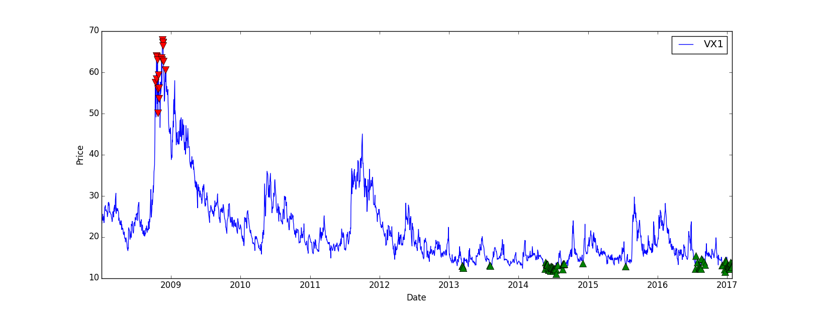
Now we’d like to visualize the signal to check if, at least, the strategy looks profitable:
# Plot the VX1, not the VIX since we're going to trade the future and not the index directly
plt.plot(data.index, data['VX1'], label='VX1')
# Plot the buy and sell signals on the same plot
plt.plot(sells.index, data.ix[sells.index]['VX1'], 'v', markersize=10, color='r')
plt.plot(buys.index, data.ix[buys.index]['VX1'], '^', markersize=10, color='g')
plt.ylabel('Price')
plt.xlabel('Date')
plt.legend(loc=0)
# Display everything
plt.show()
The result is quite good, even though there’s no trade between 2009 and 2013, we could improve that later:
Backtesting
Let’s check if the strategy is profitable and get some metrics. We’re going to compare our strategy returns with the “Buy and Hold” strategy, which means we just buy the VX1 future and wait (and roll it at each expiry), this way we can see if our strategy is more profitable than a passive one.
I put the backtest method in a separate file to make the main code less heavy, but you can keep the method in the same file:
import numpy as np
import pandas as pd

# data = prices + dates at least
def backtest(data):
cash = 100000
position = 0
total = 0

data['Total'] = 100000
data['BuyHold'] = 100000
# To compute the Buy and Hold value, I invest all of my cash in the VX1 on the first day of the backtest
positionBeginning = int(100000/float(data.iloc[0]['VX1']))
increment = 1000

for row in data.iterrows():
price = float(row[1]['VX1'])
signal = float(row[1]['Signal'])

if(signal > 0 and cash - increment * price > 0):
# Buy
cash = cash - increment * price
position = position + increment
print(row[0].strftime('%d %b %Y')+" Position = "+str(position)+" Cash = "+str(cash)+" // Total = {:,}".format(int(position*price+cash)))

elif(signal < 0 and abs(position*price) < cash):
# Sell
cash = cash + increment * price
position = position - increment
print(row[0].strftime('%d %b %Y')+" Position = "+str(position)+" Cash = "+str(cash)+" // Total = {:,}".format(int(position*price+cash)))

data.loc[data.index == row[0], 'Total'] = float(position*price+cash)
data.loc[data.index == row[0], 'BuyHold'] = price*positionBeginning

return position*price+cash
In the main code I’m going to use the backtest method like this:
# Backtest
backtestResult = int(backtest(data))
print(("Backtest => {:,} USD").format(backtestResult))
perf = (float(backtestResult)/100000-1)*100
daysDiff = (data.tail(1).index.date-data.head(1).index.date)[0].days
perf = (perf/(daysDiff))*360
print("Annual return => "+str(perf)+"%")
print()

# Buy and Hold
perfBuyAndHold = float(data.tail(1)['VX1'])/float(data.head(1)['VX1'])-1
print(("Buy and Hold => {:,} USD").format(int((1+perfBuyAndHold)*100000)))
perfBuyAndHold = (perfBuyAndHold/(daysDiff))*360
print("Annual return => "+str(perfBuyAndHold*100)+"%")
print()

# Compute Sharpe ratio
data["Return"] = data["Total"]/data["Total"].shift(1)-1
volatility = data["Return"].std()*252
sharpe = perf/volatility
print("Volatility => "+str(volatility)+"%")
print("Sharpe => "+str(sharpe))
It’s important to display the annualized return, a strategy with a 20% return over 10 years is different than a 20% return over 2 months, we annualize everything so that we can compare strategies easily. The Sharpe Ratio is a useful metric, it allows us to see if the return is worth the risk, in this example I just assumed a 0% risk-free rate, if the ratio is > 1 it means the risk-adjusted return is interesting, if it’s > 10 it means the risk-adjusted return is very interesting, basically high return for a low volatility.
In our example we have a pretty nice Sharpe ratio of 4.6 which is quite good:
Backtest => 453,251 USD
Annual return => 38.3968478261%

Buy and Hold => 53,294 USD
Annual return => -5.07672097648%

Volatility => 8.34645515332%
Sharpe => 4.60037789945
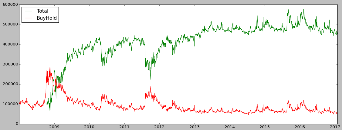
Finally, we want to plot the strategy PnL vs the “Buy and hold” PnL:
plt.plot(data.index, data['Total'], label='Total', color='g')
plt.plot(data.index, data['BuyHold'], label='BuyHold', color='r')
plt.xlabel('Date')
plt.legend(loc=0)
plt.show()
The strategy perfomed very well until 2010 but then from 2013 the PnL starts to stagnate:
Conclusion
I showed you a basic structure of creating a strategy, you can adapt it to your needs, for example you can implement your strategy using zipline instead of a custom bactktesting module. With zipline you’ll have way more metrics and you’ll easily be able to run your strategy on different assets, since market data is managed by zipline.
I didn’t mention any transactions fees or bid-ask spread in this post, the backtest doesn’t take into account all of this so maybe if we include them the strategy would lose money!